ok so there's these things called Linear Transformations & so basically what happens is you have this underlying matrix & the column vectors of the matrix represent the image of the basis vectors under the transformation
also so sometimes you can conjugate them and replace all the i's w -i's and sometimes you also transpose them which means you mirror them around the main diagonal and also the main diagonal of diagonalized matrix is the eigenvalues & if you add the main diagonal of a triangular matrix you get the determinant so that's kinda cool I guess
eigenvectors are the ones that are only scaled under tranformation, eigenvalues are the scalar multiples of the eigenvectors
ok this is me Ashley Vu officially me for real and that is all kids thanks for reading !
Friday, September 29, 2017
Tuesday, June 3, 2014
BQ #7: Unit V: Derivatives and the Area Problem
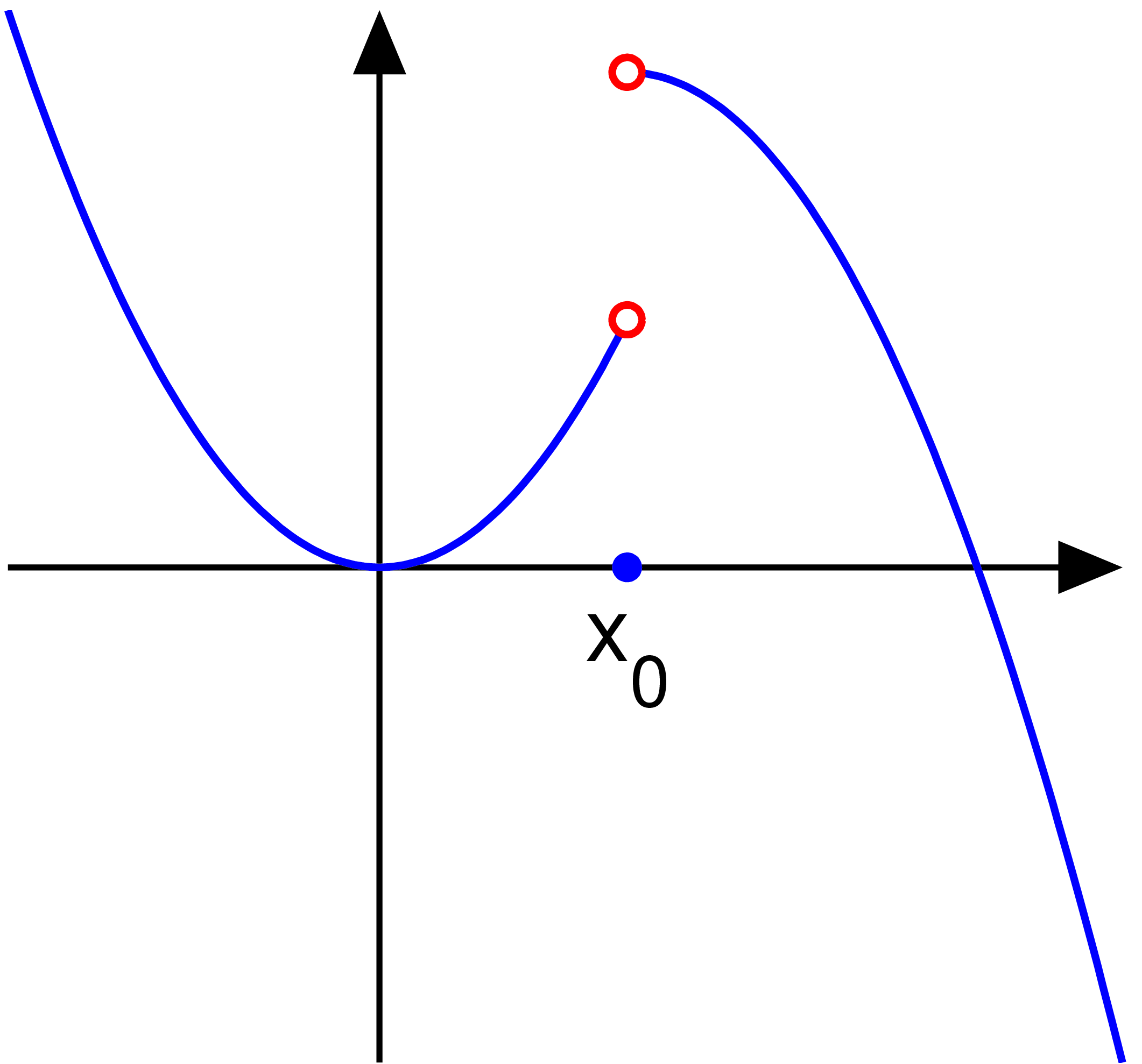
The difference quotient is a something we have come across earlier in Math Analysis. However, the question now is, how are we able to derive this? Where does this come from? Presently, with our newfound knowledge of calculus, we know that the difference quotient basically is the first step towards finding our derivative (the slope of all tangent lines). On a side note, we know that in order to find the derivative, we do the difference quotient, then find the limit of it, as h approaches 0. But again, we go back the question of how did we get the difference quotient in the first place? Look at the picture below for better clarification--I will explain below.
 |
| http://cis.stvincent.edu/carlsond/ma109/DifferenceQuotient_images/IMG0470.JPG |
I mentioned before that the derivative is basically the SLOPE of all tangent lines. When you hear slope, you should think of the formula we use to find the slope: (y-y)/(x-x) (rise over run). We are going to use this formula and basically, plug a few more things in to make it the difference quotient. In order for us to the the slope formula, we need to know two points. Look at the graph above. That first point, we will assume that the x value is just "x". Thus, the y value must be "f(x)". So, our first point is (x, f(x)). Our second point ,we move further across the x axis. We will call the distance crossed "h". So the x value would be x+h. So, it only makes sense that our y value is f(x+h). Our second point is (x+h, f(x+h)). Now that we have our two points, we will plug it in our slope formula. So your plugged in slope formula should be [f(x+h)-f(x)]/[x+h-x]. We simplify the bottom because the x's cancel out and you are left with this: [f(x+h)-f(x)]/h. THE DIFFERENCE QUOTIENT.
Now you know where the difference quotient comes from. However, in calculus, we proceed further, as I mentioned before. If you were trying to find the slope, the derivative, you would find the limit as h approaches 0. Your main question is probably why is h approaching zero. The thing is, we want to be able to find our tangent line (a line that touches the graph at one point). The problem is that we a secant line, where we touch the graph TWICE (as you can see the red line is touching the blue line twice in the picture above). So, in order for us to get one point, we can basically have those two points on top of each other... meaning that they are in the same place. We are able to get them to sit on top of each other by decreasing the "h", the distance between the two points. The smaller "h" is the closer the two points are. Therefore, we have our limit as h approaches 0 because we can't actually have it at 0, but we can get it pretty darn close.
This is just a hint of what calculus has in store, and I'm still waiting for the rest to be revealed! This is my final blogpost and I hope these posts have helped in some way or another because I know I've learned a lot this year. I've conquered Math Analysis and no lie... I feel like a Mathematician. I'm done! Lights out. *Nox*
References:
http://cis.stvincent.edu/carlsond/ma109/DifferenceQuotient_images/IMG0470.JPG
Sunday, May 18, 2014
BQ #6 - Unit U
1. What is continuity? What is discontinuity?
With functions in real life, we deal with both continuity and discontinuity. Continuous graphs entail of many characteristics: predictability (meaning you are able to know where the graph is going), the lack of breaks, holes, and jumps (because it is CONTINUOUS), and the ability to be drawn without lifting your pencil. Knowing this, we can also note that in a continuous graph, all limits should be equivalent to its values (if this is not completely understood, it will be clearer with further information). Basically, continuity is seen in many of the graphs dealt with in earlier years of math (in regular parabolas, linear graphs, etc).
Discontinuity is the opposite, as you can already guess. Discontinuous graphs have breaks, jumps, and holes, meaning you WILL need to lift your pencil from the paper in order to draw these graphs. There are four specific discontinuities found in these types of graphs. The four discontinuities branch into two categories: removable and non-removable. The only discontinuity that is removable is a point discontinuity. These occur when we have a hole in the graph.
There are three non-removable discontinuities: jump discontinuity, oscillating behavior, and infinite discontinuity. Jump discontinuities occur when our left and right limits do not match. Look at the picture below to understand this better.
Oscillating behavior occurs wherever you see "wiggles".
Infinite discontinuity occurs when a vertical asymptote is present which leads to unbounded behavior.
2. What is a limit? When does a limit exist/not exist? What is the difference between a limit and a value?
The limit does not exist at those three non-removable discontinuities we discussed earlier. The question though is why? The limit does not exist at a jump discontinuity because we have different left, right limits, as I said before. When I say this, I mean that the left and right sides of the function just don't match up; they do not meet the same INTENDED height. It is as if you and your friend went to two different diners, you didn't meet up with each other. With jump discontinuities, because the limit does not exist, we have side limits, our left and right limits that I mentioned before. These side limits look practically the same as our limit notation (the limit as x approaches a # of f(x) is equal to L)  (http://webpages.charter.net/mwhitneyshhs/calculus/limits/limit01.jpg). The only difference is that our side limits have a (+) and (-) next to that c, our number. A c- is from the left limit; a c+ is from the right limit.
Moving on, the limit does not exist when dealing with oscillating behavior. It is practically impossible to actually see the limit of this graph (because of so many wiggles). Truthfully, it does not approach a single value.
I used this picture below but it provides a good example of a limit and a value that are different. The hole in the graph is our limit. Why? Take your fingers and place one to the left and one to the right of the graph. Inch them closer and closer to one another. Notice how they INTEND to reach the hole. They intend to reach that hole, therefore, that is our limit. However, above that hole, we have an actual point, our VALUE because it is the ACTUAL height of the function.
Graphically, we take our left and right finger and basically trace ourselves. We first plug our function into the y=screen of our graphing calculator. Then, we go to GRAPH and we TRACE. We trace to the value we are looking for basically.
Sometimes, we are actually given a graph. If this occurs, you place your figners to the left and right of where you want to evaluate a limit. Wherever your fingers meet, you have a limit. If they do not meet, your limit does not exist. The video below shows better visual for this process.
Finally, we can evaluate limits algebraically. There are three ways to do this; direct substitution, dividing/ factoring out, and rationalizing/ conjugate.
Direct substituion is where we basically take the x value that we are approaching and plug it into the function. There are four possibilities. You could end up with a numerical answer, 0/# (still 0), #/0 (undefined, which means the limit does not exist), and 0/0 which is indeterminate form. If you ever get indeterminate form, you use another method.
The dividing out/ factoring method is used when we get indeterminate form. What we do here is factor what we can. If you get x^2-9 you factor that into (x-3)(x+3), and other things of that sort (sum and difference of cubes will pop up as well). If factored correctly, you should be able to cancel something out. After canceling out terms, you should be left with a simpler function. Plug in the number that you are approaching and you should get your answer.
Rationalizing/ conjugate method is used if you cannot factor out--most likely, you have a radical. All you need to do is multiply the entire fraction by the conjugate. You take the conjugate of the term that has the radical. (If you do not know what the conjugate is, it is basically changing it from say this: 3x+1 to this: 3x-1. You just change the sign). You should be able to cancel terms out after FOILing. Plug the number into the simplified problem and you get your answer.
In the video below, they go over examples of the three ways to algebraically solve limits. (The video is a little shaky, but the content is there).
References:
1.http://dj1hlxw0wr920.cloudfront.net/userfiles/wyzfiles/4a69dec7-03e0-492f-ac16-4dcd555579c9.gif
2. http://upload.wikimedia.org/wikipedia/commons/e/e6/Discontinuity_jump.eps.png
3. http://webpages.charter.net/mwhitneyshhs/calculus/limits/limit-graph8.jpg
4. http://dj1hlxw0wr920.cloudfront.net/userfiles/wyzfiles/44bad38c-431e-4382-8fe9-86303561b2a0.gif
5. http://media.tumblr.com/tumblr_m1eqlrQcTf1qdt09k.gif
6. http://webpages.charter.net/mwhitneyshhs/calculus/limits/limit01.jpg
7. http://www.vias.org/calculus/img/03_continuous_functions-69.gif
8. https://www.youtube.com/watch?v=8z4aofW85K4
9. https://www.youtube.com/watch?v=aVcqrDFcaCA
10. https://www.youtube.com/watch?v=CvB4080WC48
With functions in real life, we deal with both continuity and discontinuity. Continuous graphs entail of many characteristics: predictability (meaning you are able to know where the graph is going), the lack of breaks, holes, and jumps (because it is CONTINUOUS), and the ability to be drawn without lifting your pencil. Knowing this, we can also note that in a continuous graph, all limits should be equivalent to its values (if this is not completely understood, it will be clearer with further information). Basically, continuity is seen in many of the graphs dealt with in earlier years of math (in regular parabolas, linear graphs, etc).
Discontinuity is the opposite, as you can already guess. Discontinuous graphs have breaks, jumps, and holes, meaning you WILL need to lift your pencil from the paper in order to draw these graphs. There are four specific discontinuities found in these types of graphs. The four discontinuities branch into two categories: removable and non-removable. The only discontinuity that is removable is a point discontinuity. These occur when we have a hole in the graph.
 |
| Point Discontinuity (http://dj1hlxw0wr920.cloudfront.net/userfiles/wyzfiles/4a69dec7-03e0-492f-ac16-4dcd555579c9.gif) |
 |
| Jump Discontinuity (http://upload.wikimedia.org/wikipedia/commons/e/e6/Discontinuity_jump.eps.png) |
 |
| Oscillating behavior (http://webpages.charter.net/mwhitneyshhs/calculus/limits/limit-graph8.jpg) |
 |
| Infinite Discontinuity (http://dj1hlxw0wr920.cloudfront.net/userfiles/wyzfiles/44bad38c-431e-4382-8fe9-86303561b2a0.gif) |
A limit is the intended height of the graph. Think of it as where the left and right are intended to meet. You and your friend are meeting at a diner but come from different ways. As long as the two sides meet, your limit exists. Let's go further into this. We now know what a limit is but where does the limit exist and where does it not.
I mentioned briefly in the section above about limits. In continuous graphs, the limit always exists because the graph continuously intends to reach the same point. Let's go into our discontinuities again. Looking back at the point discontinuity, understand that our limit does exist here despite the hole present. Remember, a limit is the INTENDED height, meaning we intended to get there. A hole marks the place that we intended to get to. Think of it like you and your friend tried to meet at the diner but the diner moved somewhere else. You two still should have ended up at the same place.
Now, sometimes...
 |
| I'm sorry, I had to. (http://media.tumblr.com/tumblr_m1eqlrQcTf1qdt09k.gif) |
(http://webpages.charter.net/mwhitneyshhs/calculus/limits/limit01.jpg). The only difference is that our side limits have a (+) and (-) next to that c, our number. A c- is from the left limit; a c+ is from the right limit.  |
| One Sided Limits (right limit, top; left limit, bottom) (http://www.vias.org/calculus/img/03_continuous_functions-69.gif) |
Finally, the limit does not exist when we have an infinite discontinuity. As stated before, this discontinuity exists when we have a vertical asymptote which leads to unbounded behavior. This basically means that it is approaching infinity but really, we can never approach infinity because it is not an actual numerical value. That is why our limit does not exist.
Just to clarify as well, we understood earlier that a limit is the INTENDED height of a function. Therefore, it is good to know that the value is the ACTUAL height of a function.
|
| (http://dj1hlxw0wr920.cloudfront.net/userfiles/wyzfiles/4a69dec7-03e0-492f-ac16-4dcd555579c9.gif) |
I mentioned this before though, our limit and value are not always different. In continuous graphs, our point where we intend to reach (the limit) is also the actual value of the graph.
3. How do we evaluate limits numerically, graphically, and algebraically?
We use tables to evaluate limits numerically. We take a limit and find x values that approach it and find out. You want to find 3 values to the left of the value and 3 to the right. From there, you would trace these x values (in your graphing calculator) and find the y value. By finding the y values you should notice whether or not they are approaching each other towards a common limit or not. For better understanding, watch the video below, as they go over it more in depth.
Graphically, we take our left and right finger and basically trace ourselves. We first plug our function into the y=screen of our graphing calculator. Then, we go to GRAPH and we TRACE. We trace to the value we are looking for basically.
Sometimes, we are actually given a graph. If this occurs, you place your figners to the left and right of where you want to evaluate a limit. Wherever your fingers meet, you have a limit. If they do not meet, your limit does not exist. The video below shows better visual for this process.
Finally, we can evaluate limits algebraically. There are three ways to do this; direct substitution, dividing/ factoring out, and rationalizing/ conjugate.
Direct substituion is where we basically take the x value that we are approaching and plug it into the function. There are four possibilities. You could end up with a numerical answer, 0/# (still 0), #/0 (undefined, which means the limit does not exist), and 0/0 which is indeterminate form. If you ever get indeterminate form, you use another method.
The dividing out/ factoring method is used when we get indeterminate form. What we do here is factor what we can. If you get x^2-9 you factor that into (x-3)(x+3), and other things of that sort (sum and difference of cubes will pop up as well). If factored correctly, you should be able to cancel something out. After canceling out terms, you should be left with a simpler function. Plug in the number that you are approaching and you should get your answer.
Rationalizing/ conjugate method is used if you cannot factor out--most likely, you have a radical. All you need to do is multiply the entire fraction by the conjugate. You take the conjugate of the term that has the radical. (If you do not know what the conjugate is, it is basically changing it from say this: 3x+1 to this: 3x-1. You just change the sign). You should be able to cancel terms out after FOILing. Plug the number into the simplified problem and you get your answer.
In the video below, they go over examples of the three ways to algebraically solve limits. (The video is a little shaky, but the content is there).
References:
1.http://dj1hlxw0wr920.cloudfront.net/userfiles/wyzfiles/4a69dec7-03e0-492f-ac16-4dcd555579c9.gif
2. http://upload.wikimedia.org/wikipedia/commons/e/e6/Discontinuity_jump.eps.png
3. http://webpages.charter.net/mwhitneyshhs/calculus/limits/limit-graph8.jpg
4. http://dj1hlxw0wr920.cloudfront.net/userfiles/wyzfiles/44bad38c-431e-4382-8fe9-86303561b2a0.gif
5. http://media.tumblr.com/tumblr_m1eqlrQcTf1qdt09k.gif
6. http://webpages.charter.net/mwhitneyshhs/calculus/limits/limit01.jpg
7. http://www.vias.org/calculus/img/03_continuous_functions-69.gif
8. https://www.youtube.com/watch?v=8z4aofW85K4
9. https://www.youtube.com/watch?v=aVcqrDFcaCA
10. https://www.youtube.com/watch?v=CvB4080WC48
Sunday, April 20, 2014
BQ#4 – Unit T Concept 3
Why is a “normal” tangent graph uphill, but a “normal” Cotangent graph downhill? Use unit circle ratios to explain.
Asymptotes play such a large part in the reason why "normal" tangent graphs go up and why "normal" cotangent graphs go down.
Tangent, as discussed before, has the ratio of y/x or sine/cosine. With this knowledge, we know that whenever our x-value/cosine is 0, we will have an asymptote. Well, if we think about it, at pi/2 (0,1) and 3pi/2 (0,-1), our x-value is 0. These are where are asymptotes lie. Now, thinking back to our unit circle, we know that from pi/2 to pi, we go into Quadrant II, where only sine is positive--in other words, tangent is negative. So, in our first half of the space between our two asymptotes, our values are negative. Moving on, we know that pi to 3pi/2 in the unit circle is Quadrant III where tangent is positive. So, our other half of the space between our two asymptotes is going to be positive. Looking at the entire picture, we would see that our tangent graph begins at the bottom and goes up, making it uphill!
Cotangent has the same idea. Its ratio is x/y or cosine/sine. We want sine/our y-value to be 0 in order to find our asymptotes. So, the only places in the unit circle where we have 0 as our y-value are at 0 radians (1,0) and pi (-1,0). Therefore, our asymptotes are at 0 and pi. Again--same idea. From 0 to pi/2, we have Quadrant I where all trig functions are positive; cotangent is positive. However, from pi/2 to pi, we have only sine being positive so cotangent is negative. Guess what? That is what we are going to be seeing on our cotangent graph. Our first half of the space between the asymptotes is basically Quadrant I, so our graph will have positive values. However, our second half of the period is in Quadrant II where we established the fact that cotangent is negative. Our graph will go down. So, looking at the entire graph as a whole, we see that our graph starts from top to bottom, going downhill.
.JPG)
Asymptotes play such a large part in the reason why "normal" tangent graphs go up and why "normal" cotangent graphs go down.
Tangent, as discussed before, has the ratio of y/x or sine/cosine. With this knowledge, we know that whenever our x-value/cosine is 0, we will have an asymptote. Well, if we think about it, at pi/2 (0,1) and 3pi/2 (0,-1), our x-value is 0. These are where are asymptotes lie. Now, thinking back to our unit circle, we know that from pi/2 to pi, we go into Quadrant II, where only sine is positive--in other words, tangent is negative. So, in our first half of the space between our two asymptotes, our values are negative. Moving on, we know that pi to 3pi/2 in the unit circle is Quadrant III where tangent is positive. So, our other half of the space between our two asymptotes is going to be positive. Looking at the entire picture, we would see that our tangent graph begins at the bottom and goes up, making it uphill!
Cotangent has the same idea. Its ratio is x/y or cosine/sine. We want sine/our y-value to be 0 in order to find our asymptotes. So, the only places in the unit circle where we have 0 as our y-value are at 0 radians (1,0) and pi (-1,0). Therefore, our asymptotes are at 0 and pi. Again--same idea. From 0 to pi/2, we have Quadrant I where all trig functions are positive; cotangent is positive. However, from pi/2 to pi, we have only sine being positive so cotangent is negative. Guess what? That is what we are going to be seeing on our cotangent graph. Our first half of the space between the asymptotes is basically Quadrant I, so our graph will have positive values. However, our second half of the period is in Quadrant II where we established the fact that cotangent is negative. Our graph will go down. So, looking at the entire graph as a whole, we see that our graph starts from top to bottom, going downhill.
Friday, April 18, 2014
BQ#3 – Unit T Concepts 1-3
How do the graphs of sine and cosine relate to each of the others? Emphasize asymptotes in your response.
Sine and cosine are found in the ratio identities of the rest of the four trig functions; they affect each one of those trig functions because of this.
Tangent
With tangent, we know that tangent is equal to sine over cosine. Now, just by knowing the values of sine and cosine, we can assume what tangent will be on the graph. Look at the visual below to better your understanding.
If you look at the red highlighted area, that is 0 to pi/2, so basically the first quadrant. Even without looking at this graph, we know that sine and cosine are positive, so tangent must be positive as well (positive divided by a positive is a positive). And you can see this translate on the graph. If you look at the green cosine values and the red sine values, you can tell they are above the x-axis, meaning they are positive. And, we determined that since those to trig functions are positive, tangent must be positive, which it is (the orange line). You can see the same thing going on in the next parts of the graph. In the "Quadrant II", on the graph, you can tell that cosine is negative (as the green values fall below the x-axis) and sine is positive (as the red values are above the x-axis). And because of our ratio identity of tan(x)=sin(x)/cos(x), we know that a positive divided by a negative makes a negative. That is why the tangent values fall below the x-axis this time. The 3rd quadrant, again, look at our sine and cosine values: they are both negative. So, a negative divided by a negative is a positive: tangent values are positive. Finally, you should be understanding the relationship that tangent, cosine, and sine have. The last part of the period, cosine is positive (values are above the x-axis) and sine is negative (values below the x-axis); tangent is negative.
Cotangent has the same thing going on as we saw in tangent. Remember to look at the values of the sine and cosine graphs and relate them to cotangent. For example, see how sine and cosine values are positive, so we have cotangent as positive. However, in the green section, we see that sine (the red graph) has positive values and cosine (green graph) has negative values; we can deduce that cotangent is negative because a negative divided by a positive is a negative.
Sine and cosine are found in the ratio identities of the rest of the four trig functions; they affect each one of those trig functions because of this.
Tangent
With tangent, we know that tangent is equal to sine over cosine. Now, just by knowing the values of sine and cosine, we can assume what tangent will be on the graph. Look at the visual below to better your understanding.
 |
| (https://www.desmos.com/calculator/cwdr1eyszr) |
Now, that you know why the tangent graph looks as it does (through the understanding of its relationship with sine and cosine), we need to deal with another part of these graphs: the asymptotes. The asymptotes are not just there because we say so. There is a reason behind it. Remember when we talked about how tan(x)=sin(x)/cos(x)? We are using this identity again. We know that asymptotes are created when we have an undefined value. We get undefined values when we divide by 0. So, knowing that... we look to our ratio identity and see that cosine must equal 0 in order to get an undefined value (because we are dividing by cosine). How do we get cosine to equal 0? Well, we know that cosine is essentially the x-values of certain points in our unit circle. The only parts of the unit circle that have 0 as an x-value are pi/2 (0,1)and 3pi/2 (0, -1). Therefore, these marks on the graph are where we have asymptotes! Look at the graph above and see where it seems like the tangent graph discontinues; do you notice that pi/2 and 3pi/2 are where we don't really see the tangent graph go? That is because of the asymptotes!
Cotangent
Cotangent has sine and cosine in its ratio identity as well. Cot(x)=cos(x)/sin(x).
 |
| (https://www.desmos.com/calculator/cwdr1eyszr) |
Because cotangent has a different ratio than tangent, we are going to be having some different ratios. The ratio identity of cotangent is cot(x)=cos(x)/sin(x). Again, asymptotes are undefined values, meaning they are divided by 0. So, because sine is our denominator in this ratio, sine must be equal to 0 in order to find asymptotes. Where on our unit circle do we have sine=0? Sine is y/r, basically the y values of the unit circle. So, we know the only parts of the unit circle where the y values are 0 are 0 (1,0) and pi (-1,0). Knowing this, we know that our asymptotes are at 0 radians and pi. Look at the graph above and check to make sure. Notice how at 0 radians, a new period begins, as if we lifted our pencil to create a new part of the graph. The same is seen at the pi mark.
Secant
Secant is a little different from tangent and cotangent. Its ratio identity is 1/cos(x).
 |
| (created at https://www.desmos.com/calculator) |
We have the same idea though, as we saw in the previous graphs. If cosine is negative, then secant values must be negative as well. If cosine is positive, the secant graph must be positive as well. You can see this in the graph. The cosine values (the black graph) are positive in the red shaded part of the graph; and look at that, the secant graph (the red graph) is positive in that section as well. You can see the trend in the following sections/quadrants as well. It is good to remember that the sine values in here do not have any effect on the secant graph because it is not part of its ratio (*disregard the orange sine graph in the picture above*).
The asymptotes of secant are the same as we saw in tangent. Tangent had cosine as the denominator as well. So, we know that at pi/2 (0,1) and 3pi/2 (0,-1) there are going to be asymptotes for this secant graph.
Cosecant
Cosecant has the same idea as secant just reversed, like we saw with cotangent and tangent. Cosecant's ratio identity is csc(x)=1/sin(x).
 |
| (created at https://www.desmos.com/calculator) |
Again, we remember that if sine is positive on the graph, then cosecant must be positive as well, because 1 divided by a positive is always a positive--and vice versa. You can see in the red shaded part, the sine graph (the orange line) is positive and the cosecant graph (the red line) is positive as well. It is good to remember that cosine has no effect on cosecant because it is not found in the ratio (*therefore, disregard the cosine graph in the picture above*).
Cosecant has its asymptotes wherever sine is 0 (because we are dividing by sine in this ratio). Looking back to our cotangent graph, we remember that sine was 0 at 0 radians and pi (because of the coordinates of (1,0) and (-1,0)). So, we will have cosecant's asymptotes at 0 radians and pi. That is why, if you look at the picture above, you see that the graph seems to cut out at 0 radians and pi.
Thursday, April 17, 2014
BQ#5 – Unit T Concepts 1-3
Why do sine and cosine NOT have asymptotes, but the other four trig graphs do? Use unit circle ratios to explain.
Sine and cosine do not have asymptotes because their ratios are y/r and x/r, meaning that the radius will ALWAYS be the denominator. You will never have a 0 as your denominator. Because of this, we will never encounter an undefined answer, meaning we will not encounter any asymptotes (since asymptotes = undefined, basically).
However, that is a different case for cosecant, secant, cotangent, and tangent. Cosecant has a ratio of r/y. The "y" value can be 0 in certain cases: if we are at (1,0) or (-1,0). Same for secant; secant has a ratio of r/x and x can be 0 in some cases: (0,1) and (0, -1). Cotangent and tangent have the ratios of x/y and y/x so, again, of course you will have some y values and x values that equal to 0.
Also, a good thing to nice is that cotangent and and cosecant have the same denominator in their ratios: y. Therefore, they will have the same asymptotes. Tangent and secant will have the same asymptotes as well because their denominators in their ratios are x.
Wednesday, April 16, 2014
BQ#2 – Unit T Concept Intro
How do the trig graphs relate to the unit circle?
Trig graphs, believe it or not, are essentially the unit circle unwrapped (at least in one period). BAM. Let's think about what we already know about the unit circle. We are going to use sine as an example, first. In the case of sine, the 1st and 2nd quadrants are positive whereas the 3rd and 4th quadrants are negative. Now, the 1st quadrant goes from 0 radians to pi/2. The 2nd quadrant goes from pi/2 and pi. So from this information alone, we can deduce that from 0 to pi, our values are going to be POSITIVE. The 3rd quadrant goes from pi to 3pi/2; the 4th goes from 3pi/2 to 2pi. Because sine is negative in these quadrants on the unit circle, in the trig graphs, from pi to 2pi, our values are going to be negative. Thus, the whole entire graph will go up and then down, because it is corresponding with the values we know from the unit circle.
.JPG)
Trig graphs, believe it or not, are essentially the unit circle unwrapped (at least in one period). BAM. Let's think about what we already know about the unit circle. We are going to use sine as an example, first. In the case of sine, the 1st and 2nd quadrants are positive whereas the 3rd and 4th quadrants are negative. Now, the 1st quadrant goes from 0 radians to pi/2. The 2nd quadrant goes from pi/2 and pi. So from this information alone, we can deduce that from 0 to pi, our values are going to be POSITIVE. The 3rd quadrant goes from pi to 3pi/2; the 4th goes from 3pi/2 to 2pi. Because sine is negative in these quadrants on the unit circle, in the trig graphs, from pi to 2pi, our values are going to be negative. Thus, the whole entire graph will go up and then down, because it is corresponding with the values we know from the unit circle.
As you see, the same can be seen for other trig functions. For cosine, we have the pattern being positive, negative, negative, postive. Therefore, on the graph, you will see the period beginning with positive values, but dipping at pi/2 and becoming negative. At pi, it remains negative, but when you hit the mark of 3pi/2, our values will be positive, as it should.
Tangent and cotangent are similar however there is a special situation with them (which I will go into further detail in the next section). Anyway, our graph for tangent/cotangent will begin with positive values, then negative values, then positive, and negative. However, if you notice, we have a pattern already seen in the first two quadrants, that is then repeated in the next two quadrants--which leads us into the next question!
Period? - Why is the period for sine and cosine 2pi, whereas the period for tangent and cotangent is pi?
The period for sine and cosine is 2pi because the pattern finishes at 2pi and does not repeat until we begin another "revolution" around the unit circle. The pattern is +,+,-,- for sine. The pattern is +, -, -, +. You see, you need all quadrants in order to explain the FULL pattern. You need to go around the unit circle in ONE FULL revolution. So, your period will go to 2pi.
The period for sine and cosine is 2pi because the pattern finishes at 2pi and does not repeat until we begin another "revolution" around the unit circle. The pattern is +,+,-,- for sine. The pattern is +, -, -, +. You see, you need all quadrants in order to explain the FULL pattern. You need to go around the unit circle in ONE FULL revolution. So, your period will go to 2pi.
The period for tangent and cotangent is only pi. Why? Look at the picture above. Do you notice that the pattern is +, -, +, -? The pattern repeats itself twice in one revolution of the unit circle. Why do we want to repeat that? So, we only really need the first quadrant in order to fully explain the pattern. That is why tangent and cotangent periods only go to pi.
Amplitude? – How does the fact that sine and cosine have amplitudes of one (and the other trig functions don’t have amplitudes) relate to what we know about the Unit Circle?
So why is it that we have amplitudes of one for sine and cosine? Think about it. Sine has the ratio of y/r. Cosine has the ratio of x/r. R can only equal 1, since the radius of a unit circle has to be 1. So, the values x and y can only go up to 1 themselves. So if you can only divide 1 by 1 to get the largest number... your largest value can only be 1/ -1. That is why sine and cosine cannot equal something greater than 1 or less than -1. However, think about the other trig functions and their ratios. Tangent is y/x. You are not restricted to values between -1 and 1 because you are dividing by different numbers that vary from being just 1 and -1. Same is for cotangent but backwards. Also, for trig functions like cosecant and secant, you have r/y and r/x. You can divide your "r" (1) by a small number like 1/2 and end up with 2. That is why those other funcitons do not have amplitudes.
Subscribe to:
Comments (Atom)